
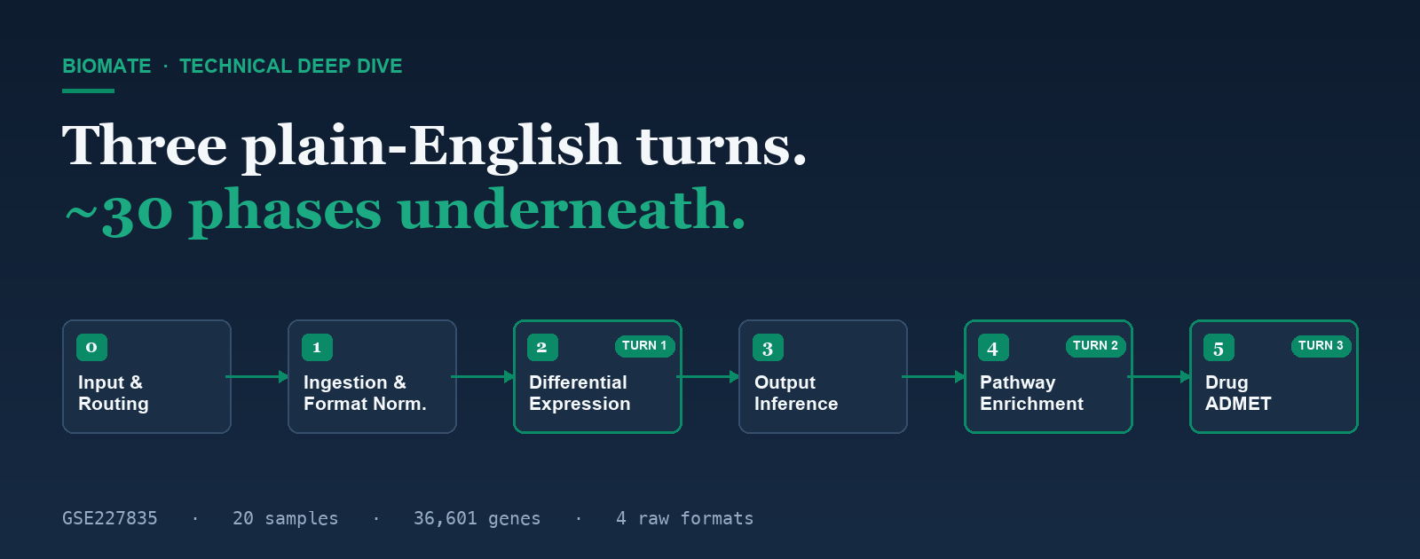
On the summit stage, BioMate turns a real myasthenia gravis dataset into a developability verdict in three plain-English turns. That is the surface. Underneath, those three turns fan out into roughly thirty discrete phases — format detection, pseudobulk aggregation, robust dispersion estimation, output inference, enrichment, and ADMET. This is the companion to the demo announcement: the engineering, phase by phase, with the real numbers from the run.
The Hard Part Was Never the Statistics — It Was the Raw Data
Every public dataset arrives in the shape its depositor happened to use. Most bioinformatics tools quietly assume one canonical layout — usually 10x Genomics matrix bundles — and simply fail on anything else. The case for this demo, GSE227835 (single-cell RNA-seq of AChR+ myasthenia gravis vs. healthy controls), ships as dense per-sample expression tables — one gzipped genes×cells matrix per subject — not the matrix.mtx/barcodes.tsv/features.tsv triplet most pipelines expect. A tool that only reads 10x MEX would stop before computing a single statistic.
BioMate’s ingestion layer detects and normalizes four distinct raw-data shapes automatically:
matrix.mtx.gz + barcodes + features per sample..tar.gz per subject that unpacks to MEX files.Whichever shape it finds, the ingestion workflow pseudobulk-aggregates the single-cell counts up to the sample level, harmonizes the metadata, auto-detects the condition and contrast, and emits three DESeq2-ready files — counts_matrix.csv, sample_metadata.csv, and contrasts.csv. The user never sees any of it. They asked one question.
Six Stages, ~30 Phases, Three Turns
Here is the complete flow. The three conversational turns map onto Stages 2, 4, and 5; Stages 0, 1, and 3 run invisibly around them.
- Input intake — accepts a GEO/SRA accession, a download link, a file upload, or a typed question.
- Accession & intent detection — recognizes
GSE/GSM/SRApatterns and the analytical intent. - Routing decision — single workflow, a suggested multi-step chain, or a disambiguation question.
- Parameter prefill — rule-based + LLM hybrid; auto-fills the accession and defaults.
- GEO fetch — retrieve the series matrix and supplementary files.
- Format detection — branch across the four shapes above (bulk / MEX / tarball / dense TSV).
- Download & extract — pull and unpack the raw archive for single-cell paths.
- Per-sample read — sparse
readMMfor MEX, dense table read for TSV. - Pseudobulk aggregation — sum counts per gene per sample, with a minimum-cells filter.
- Gene alignment — intersect the gene set across all samples.
- Metadata harmonization — auto-detect the condition column (disease vs. control).
- Contrast auto-detection — choose reference and target groups.
- Emit DESeq2-ready CSVs — counts matrix, sample sheet, contrasts.
- Stage inputs — move data from object storage onto the compute worker.
- Load & coerce — integer coercion, missing-value clamp.
- Gene filtering — drop low-count genes below the expression floor.
- Robust dispersion & test — size factors, then a parametric → local → gene-wise dispersion fallback so small or low-variance cohorts never dead-end, then the Wald test.
- Results & significant genes — ranked table plus the significant-gene list.
- Diagnostics — volcano and PCA plots.
- QC metrics & gate — evaluated against configured thresholds.
- Output resolution — locate result files across the publish directory and work directory.
- Findings generation — read the result tables and summarize the key numbers in plain English.
- Report assembly — a cited, reproducible methods-and-results record.
- Gene-list input & ID mapping — map symbols to ENTREZ identifiers.
- Over-representation analysis — enrichGO across Gene Ontology terms.
- Simplify — collapse redundant terms.
- Visualization — barplot, dotplot, cnetplot, emapplot, goplot.
- Results & findings — enriched-term table, back through Stage 3.
- Molecule input — a candidate SMILES (here, iptacopan).
- ADMET prediction & gates — clearance, hERG, CNS permeability, hepatotoxicity, with QC thresholds — then Stage 3 findings.
Live progress streaming (per phase and step), usage metering, durable run-state so long jobs survive worker restarts, and an automatic QC remediation loop — all running alongside the six stages above.
What Actually Came Out of GSE227835
Nothing below is illustrative. These are the numbers from the pipeline on the real deposit — the biology is the data’s, not the slide’s.
| Stage | Quantity | Value |
|---|---|---|
| Ingestion | Samples pseudobulked (MG + HC) | 20 |
| Ingestion | Genes per sample | 36,601 |
| Ingestion | Cells per sample | ~5,800–8,600 |
| Differential expression | Genes tested (non-NA) | 14,722 |
| Differential expression | DE genes at padj < 0.05 | 883 |
| Enrichment | DE genes GO-mappable | 99 / 141 |
| Enrichment | Lead signature | TNF-response (GO:0071356) |
The top differentially expressed genes — MCRS1, ANKRD49, NRTN, ETV7, TIGIT, BATF3, GBP1 — and the enriched cellular response to tumor necrosis factor term (padj ≈ 0.02) point to an inflammatory signature in this cohort. That is a genuine, reproducible readout of a public dataset — surfaced by asking a question in English.
Two Real Data Connections, One Mechanistic Hypothesis
It matters to be precise about what is automated data flow and what is scientific reasoning:
- Stage 1 → Stage 2 (data-connected). The pseudobulk workflow’s three CSVs are the exact inputs to differential expression. No hand-editing.
- Stage 2 → Stage 4 (data-connected). The differential-expression gene list is the exact input to enrichment.
- Stage 4 → Stage 5 (mechanistic hypothesis). The candidate drug is chosen on established biology — complement is a validated axis in AChR+ MG, and iptacopan is a clinically established complement-directed therapeutic. The ADMET assessment is a real computation; the selection of the molecule is a scientist’s hypothesis, not an output of the enrichment step.
Because a platform that blurs “the model computed this” with “a human reasoned this” is not one you can build a regulatory submission on. Every step in the pipeline is logged, cited, and reproducible — and the one step that is a hypothesis is labeled as a hypothesis.
The Engineering Is the Product
Three plain-English turns are what the audience sees. The value is in the thirty phases they don’t: the format branch that reads a dataset other tools skip, the dispersion fallback that keeps a small cohort from dead-ending, the output inference that turns a results table into a sentence. That machinery is what turns “we have a public dataset somewhere” into “here is a cited, QC-gated, reproducible answer” — without a two-week wait in the bioinformatics queue.
See it live at the summit, or start from your own accession at www.biomate.ai.